Demo: Binary Classification
Create an initial dataset for a binary classification problem with 20 features:
6 of the features are informative
4 of the features are linear combinations of the informative features
10 of the features are just random noise
[1]:
# Ignore lightgbm warnings
import warnings
warnings.filterwarnings("ignore")

# Import necessary libraries for the demo
import pandas as pd
from lightgbm import LGBMClassifier
from sklearn.datasets import make_classification
from sklearn.model_selection import train_test_split
from shapfire import ShapFire, RefitHelper, plot_roc_curve

X, y = make_classification(
    n_samples=1000,
    n_features=20,
    n_informative=6,
    n_redundant=4,
    n_repeated=0,
    n_classes=2,
    random_state=0,
    shuffle=False,
)
X = pd.DataFrame(data=X, columns=[f"feature{i}" for i in range(X.shape[1])])
X
[1]:
| feature0 | feature1 | feature2 | feature3 | feature4 | feature5 | feature6 | feature7 | feature8 | feature9 | feature10 | feature11 | feature12 | feature13 | feature14 | feature15 | feature16 | feature17 | feature18 | feature19 | |
|---|---|---|---|---|---|---|---|---|---|---|---|---|---|---|---|---|---|---|---|---|
| 0 | -0.056717 | -0.493931 | 1.667702 | 1.397865 | -0.794842 | -0.682968 | -0.511378 | -0.992701 | -0.248595 | -1.676577 | 1.206354 | 2.321515 | -1.423698 | -0.433072 | 0.682042 | -1.125577 | -0.593864 | -0.024779 | 1.735459 | -1.113934 |
| 1 | 1.012914 | -0.696091 | 0.414157 | 0.567214 | 0.729235 | 2.892775 | -0.016728 | -1.475205 | 3.680440 | -2.095504 | -0.676781 | 1.576879 | -2.227987 | 1.638134 | 0.015417 | -0.507376 | 1.178729 | 2.676799 | 0.344251 | 0.454819 |
| 2 | 1.690440 | -1.236785 | -0.507020 | 3.027518 | -2.315026 | 2.067620 | 0.273264 | 1.017970 | 1.103050 | -5.071645 | -1.156792 | -2.066161 | -1.825515 | -1.288961 | 0.324183 | 0.229208 | -0.033722 | 0.727694 | 0.745335 | -0.315728 |
| 3 | 2.035054 | -1.154556 | -0.012416 | 1.361509 | -0.931541 | 2.933542 | -0.734587 | -0.335309 | 2.853751 | -4.326141 | -0.296359 | 1.215873 | -0.278985 | -1.448467 | 0.580039 | 0.156749 | 0.639724 | 0.029043 | 0.822496 | 1.151368 |
| 4 | 1.024961 | -0.366287 | 2.079224 | 0.739798 | -0.486162 | 0.621330 | -1.945298 | -1.429361 | 1.423769 | -3.266301 | 2.028758 | -2.972793 | 0.003815 | -0.904622 | -0.139921 | -0.550930 | -1.697206 | 0.102097 | -1.056104 | 0.146621 |
| ... | ... | ... | ... | ... | ... | ... | ... | ... | ... | ... | ... | ... | ... | ... | ... | ... | ... | ... | ... | ... |
| 995 | 1.410788 | 0.250078 | 0.366037 | 1.168022 | -0.056665 | -0.251516 | -0.505207 | 0.175348 | 0.103474 | -1.987223 | -0.384352 | -1.023449 | 0.664366 | 0.745393 | 0.758317 | 1.200208 | -0.147041 | 0.158603 | -1.219479 | -1.394935 |
| 996 | -0.613218 | 1.423613 | 1.527973 | -0.245896 | -2.291340 | 0.481899 | -2.839232 | 1.633723 | -0.621871 | -3.940202 | 0.300710 | -0.307716 | -0.349721 | 0.175795 | 0.228521 | 0.212923 | 0.732526 | -0.404249 | -0.448734 | 0.305272 |
| 997 | -0.231221 | 1.140357 | -2.173634 | -1.429259 | -1.838736 | -0.198766 | -0.784890 | 3.750921 | -2.509571 | -0.128341 | -0.031324 | -0.850717 | 0.361888 | -0.409298 | 0.709181 | 1.040780 | 0.269000 | 0.130427 | -0.856227 | 0.278540 |
| 998 | -3.281446 | -1.185517 | 1.473731 | 0.117330 | -1.795964 | 1.482811 | 0.437157 | -1.201846 | 0.767806 | -0.192885 | -1.765901 | -1.326832 | -1.287806 | -0.353538 | 0.996278 | 2.046064 | -0.360873 | -0.720141 | 0.355115 | -0.995815 |
| 999 | 0.384327 | 0.535252 | -0.050257 | 0.491075 | 0.507009 | 2.607129 | 0.183923 | 0.083624 | 2.764692 | -2.048920 | -0.513324 | -0.085608 | 1.195993 | -0.924152 | -0.812521 | -0.147024 | 0.184254 | 0.145577 | 0.432219 | -0.270619 |
1000 rows × 20 columns
Dataset Split
Split the initial dataset into:
A pre-processing dataset that we use for feature ranking and selection
A final dataset which we use to obtain ROC AUC performance estimates using the selected features
[2]:
X_preprocess, X_final, y_preprocess, y_final = train_test_split(X, y, test_size=0.50, random_state=0)
Feature Importance Ranking & Selection
[3]:
# Prepare input parameters for the ShapFire method
estimator_class=LGBMClassifier
estimator_params={"objective": "binary"}
scoring="roc_auc"
n_splits = 2
n_repeats= 5
sf = ShapFire(
  estimator_class=estimator_class,
  scoring=scoring,
  estimator_params=estimator_params,
  n_splits=n_splits,
  n_repeats=n_repeats,
)

# Perform feature importance ranking and selection
_ = sf.fit(X=X_preprocess, y=y_preprocess)

# Print the selected features
# Ideally, only the 10 first features should appear in the selected features
for feature in sf.selected_features:
    print("Selected feature: ", feature)
Clustering progress 100%|=========================| 6.00/6.00 [00:00<00:00, 2.41kit/s]
ShapFire progress   100%|=========================| 20.0/20.0 [00:01<00:00, 13.0it/s]
Selected feature:  feature1
Selected feature:  feature7
Selected feature:  feature4
Selected feature:  feature0
Selected feature:  feature3
Selected feature:  feature9
Selected feature:  feature6
Selected feature:  feature8
Selected feature:  feature5
Feature Importance Plot
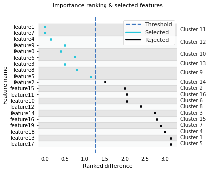
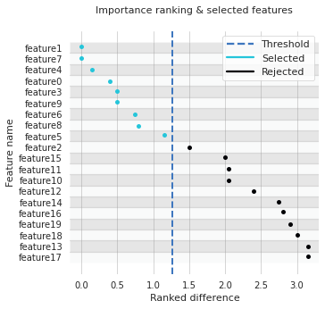
To more easily get an overview of the ranked and selected features we can plot using the ShapFire class method: plot_ranking.
[4]:
# Plot the selected features per cluster
fig, ax = sf.plot_ranking()

[5]:
# Plot the selected features per feature
fig, ax = sf.plot_ranking(groupby="feature")

Selcted Features: ROC Curves
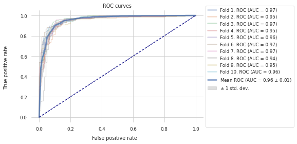
To get an unbiased estimate of the performance of a model that uses the previously selected features we can perform repeated \(k\)-fold cross-validation on the other half of the initial dataset.
[6]:
refit_helper_selected_features = RefitHelper(
    n_splits=n_splits,
    n_repeats=n_repeats,
    feature_names=sf.selected_features,
    estimator_class=estimator_class,
    estimator_params=estimator_params,
    scoring=scoring,
)
refit_helper_selected_features.fit(X_final, pd.Series(y_final))

_, _ = plot_roc_curve(df=refit_helper_selected_features.history)

All Features: ROC Curves
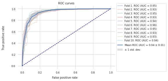
Similarly, to get an unbiased estimate of the performance of a baseline model that is trained using all initial features we perform repeated \(k\)-fold cross-validation on the other half of the initial dataset.
[7]:
refit_helper_baseline_features = RefitHelper(
    n_splits=n_splits,
    n_repeats=n_repeats,
    feature_names=X.columns.to_list(),
    estimator_class=estimator_class,
    estimator_params=estimator_params,
    scoring=scoring,
)
refit_helper_baseline_features.fit(X_final, pd.Series(y_final))

_, _ = plot_roc_curve(df=refit_helper_baseline_features.history)
